Inventor IDE Alpha 6!

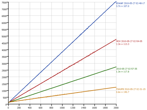
After 2 years, 1 month, and 1 day, I’m finally back in the swing of things with a new release of Inventor IDE!  Version Alpha 6 is planned to be the last major alpha release.  I will probably make a few smaller updates as 6a, 6b, etc.  It now contains the preliminary performance analysis tool, which I’ll explain in due time.  More mundane features added include Find/Replace/Find All References, and a bunch of obscure-but-problematic bugs fixed.

Plot made by the performance analysis tool in Inventor IDE Alpha 6

Jacobi eigenvalue algorithm, Schur decomposition, and Wikipedia

Me?  Writing a blog post?  Well, you see, it all started with this Wikipedia page on the “Jacobi method for complex Hermitian matrices”.  I wanted to apply the Jacobi eigenvalue algorithm to diagonalize complex matrices, since it had worked well for real symmetric matrices, but the page on it only covers real symmetric matrices, not the complex equivalent, Hermitian matrices.  I was glad to see there was the additional page supposedly explaining how to do something similar for complex Hermitian matrices, but alas, it’s explained in such complicated, ambiguous terms that it’s at best unreadable, and at worst wrong.  I implemented two different interpretations of the page’s content, and both failed on the simplest possible example…

…so I derived my own in a much simpler way, and figured out a more general algorithm.  Other people have undoubtedly found the exact same method, but papers I’d found on the topic didn’t seem to state their methods much clearer than the Wikipedia page.  The issue is that I derived it in a completely different way than what’s on Wikipedia.  It’s not a matter of “fixing a mistake” in the page; by Wikipedia’s rules, this counts as original research (despite that others have probably done the same), so it’s not allowed on Wikipedia.  The only other suggestion people had was a blog post to make sure that a correct version is online somewhere, so here it is.

In a nutshell, the Jacobi eigenvalue algorithm works by one-by-one choosing the largest off-diagonal element, and rotating the two vectors associated with that element such that the element becomes zero.  Do this enough times and all off-diagonal elements will be quite close to zero (if the matrix is Hermitian), leaving the eigenvalues.  The eigenvectors come from applying the rotations to the identity matrix.  The only thing necessary to do this is to know the eigenvectors that diagonalize a 2×2 matrix, namely

where is the matrix we’re trying to diagonalize, and is the element we’re trying to eliminate.  If is Hermitian, are real, and .  However, I won’t assume that is Hermitian, since even if it’s not, this same approach can still be used to get what’s known as the Schur decomposition, namely , where is upper triangular and the eigenvalues of are on the diagonal of .  If is Hermitian, the Schur decomposition is the same as the eigendecomposition, so .  In the non-Hermitian case, it doesn’t give the eigenvectors, but those can be more easily computed afterward.  I’ll split this into two cases.

Case 1:

This case is where you don’t have two diagonal elements that are almost identical compared to the off-diagonal element.  If you did, dividing by them could cause chaos, madness, and megalomania… or just invalid results.  We start by subtracting from our 2×2 matrix, since we’re only interested in its (pseudo-)eigenvectors , and multiples of can be diagonalized using the same eigenvectors.  That basically means that adding/subtracting multiples of won’t change .  Then, we  divide the 2×2 matrix by , which also doesn’t change the (pseudo-)eigenvectors.  This gives us

For simplicity, we’ll just relabel this as

Now, if we want to make by multiplying by a unitary matrix on the right and its conjugate transpose on the right, a bit of trial and error can give you that

is a solution to that problem.  Note that the square roots are square roots of complex numbers, not necessarily real numbers.  You can verify that this works in the original case by multiplying out and confirming that the lower off-diagonal element is zero.  If is Hermitian, both off-diagonal elements should be zero.  Case 1 complete.

Case 2:

This case is where you have two diagonal elements that are almost identical compared to the off-diagonal element.  Simple solution: pretend that they are exactly zero.  You now have

The zeros make things much simpler, as we can now find

This time, since we’ve assumed that the diagonal elements are exactly the same, it probably won’t make the off-diagonal element exactly zero, but it’ll probably be negligibly small, and if it’s ever the largest at some later point, it’ll just get picked again to be eliminated, only probably without the diagonal elements being so close the 2nd time around.

Again, you don’t have to take my word for it.  You can easily verify this solution by just multiplying it out.

How did you get these?

If you’re wondering how I figured these out (after a weekend of trial and error of different methods), I knew that if the off-diagonal element was non-zero (which it must be, else there’s nothing to do), there is some non-zero component of the second element in each vector of .  I temporarily ignored the restriction of having unit vectors and set both of those components to 1, but didn’t ignore the restriction of having the two vectors being complex orthogonal (i.e. ), giving me

I know I want that off-diagonal element zero, so

Since the scales of the 2 vectors are arbitrary, including the relative scales, I scaled one by , and the other by .  Then I just normalize them both (they happened to be the same length, ), and that’s the solution above.  I did the same for case 2, only it was even simpler.  Easy… it just took a weekend to figure out what the easy way was.

Final Algorithm to Compute Schur Decomposition

V = identity matrix
while (there is an ij such that i>j and |M[i][j]| > 10^-8*|M[i][i]-M[j][j]|) {
    select ij with maximum |M[i][j]|/|M[i][i]-M[j][j]|, possibly infinite
    // Case 1
    if (|M[i][j]| < 10^14*|M[i][i]-M[j][j]|) {
        a = 2*M[i][j]/(M[i][i]-M[j][j])
        b = 2*M[j][i]/(M[i][i]-M[j][j])
        c = sqrt(1+a*b)
        L = sqrt(|a|^2 + |1+c|^2)
        Vsub = {{1+c, -conj(a)}, {a, 1+conj(c)}}/L
    }
    // Case 2
    else {
        a = M[i][j]
        b = M[j][i]
        L = sqrt(|a|+|b|)
        Vsub = {{sqrt(b), -conj(sqrt(a))}, {sqrt(a), conj(sqrt(b))}}/L
    }
    // Rotate columns i and j of M
    for (each row of M) {
        newi = M[row][i]*Vsub[0][0]+M[row][j]*Vsub[1][0]
        newj = M[row][i]*Vsub[0][1]+M[row][j]*Vsub[1][1]
        M[row][i] = newi
        M[row][j] = newj
    }
    // Rotate rows i and j of M
    for (each column of M) {
        newi = M[i][col]*conj(Vsub[0][0])+M[j][col]*conj(Vsub[1][0])
        newj = M[i][col]*conj(Vsub[0][1])+M[j][col]*conj(Vsub[1][1])
        M[i][col] = newi
        M[j][col] = newj
    }
    // Rotate cols i and j of V
    for (each row of V) {
        newi = V[row][i]*Vsub[0][0]+V[row][j]*Vsub[1][0]
        newj = V[row][i]*Vsub[0][1]+V[row][j]*Vsub[1][1]
        V[row][i] = newi
        V[row][j] = newj
    }
}
// Diagonal of M now has the eigenvalues of the input M
// If M was Hermitian, V now has the eigenvectors of the input M as columns,
//                     in the order that the eigenvalues appear in M

More Big Software Performance Speedups

As I sit here waiting for Matlab to compute in over 25 minutes what I can now compute in 10 milliseconds in mostly-unoptimized C++ code running in debug mode, I figured I should write a blog post stressing the importance of a few small differences that can result in >150,000x speedups like this.

Note that I’m not putting down Matlab, since it’s not designed to run fast; I’m just using this as an example of why it’s important to not get complacent with performance.

1. Precomputation

This is may be the largest performance difference between the two implementations, though it might be a tight race between this and the next two differences.  Precomputation, however, is very widely applicable, easy to do, and could have been applied to the Matlab code to some extent.

The basic idea is: instead of computing the same data repeatedly, compute them once and save them.

In those words, it sounds so obvious, but it encompasses a broad range of things, some of which are less obvious.  For example, in this case, I’ve precomputed the data before running the program and read it in from input files.  I’ll be running the program using the same data possibly thousands of times, and those data took longer to compute than to read in, so there’s no sense in recomputing them each time.  In particular, I’ve computed about 1,000 points on each of a bunch of curves, and the program linearly interpolates between them, which is plenty sufficient accuracy in this case.

There are of course cases where precomputation  doesn’t make sense, such as if the computation is as fast as looking up the data or if the amount of data to save is unreasonably large, but in a very large range of applications, precomputation can speed things up a ton.

2. Native Code

People will yell until they’re blue in the face that interpreted code or Just-In-Time-compiled code is usually as fast as native code (i.e. compiled to machine code ahead of time).  They’re dead wrong, and usually somewhere up the chain, they got their information from a marketing department or a study funded by Sun, IBM, etc, even though they’re probably not aware of it.  Nonetheless, I was honestly shocked that such extremely simple tests confirm this, e.g. running the following code in Java versus in C++.

int a = 12468;
for (int i = 0; i < 2000000000; ++i) {
    a /= 2;
    a *= 2;
}
// Output a

C++ compilers trivially replace the multiplication with addition, and the division with a bit shift (and a special trick because the compiler doesn’t clue in that the value is always positive or even).  Of course, a really smart compiler would realize that the entire loop is useless, since the starting number is positive and even, but none of them appear to be that smart.  Java however, will not even do the simple replacement no matter how many times the loop is run.  This is visible by comparing against the performance of:

int a = 12468;
for (int i = 0; i < 2000000000; ++i) {
    a >>= 1;
    a += a;
}
// Output a

In Java, this new code is several times faster than the previous, whereas in C++, the performance is (almost) identical between the two, since it’s already made that replacement.

In my case today, I’m not comparing against Java; I’m comparing against Matlab, which not only doesn’t compile its code ahead of time, but literally interprets the text representing the code as it’s running, similar to VisualBasic or Fortran.  That adds factors of thousands for just figuring out what the program is doing.  It just doesn’t stand a chance outside of its prebuilt libraries.  Inside its prebuilt libraries, e.g. matrix multiplication or diagonalization code written in C++, it’s fast, so one must try to use them where reasonable.

3. Customization

As much as Matlab provides some great functionality that can be a pain in the butt to implement from scratch, such as diagonalization of big matrices, it (understandably) doesn’t let you specify everything you know that may help speed up the computation.

For example, matrix-matrix multiplication where you input two matrices and get back their product is very slow because of memory caching issues.  However, if the matrix on the right of the multiplication is already transposed ahead of time, it’s much faster.  (I’ll save the explanation of why for another time.)  Matlab doesn’t know whether there’s a way to rework your code such that some matrices are pre-transposed and others aren’t, it just receives two matrices and has to spit out the product.  If you can use your knowledge of your code to do this, you can get a big performance boost.

Another example in this case is if you have good estimates of the eigenvalues and eigenvectors of the matrix you’ve got, it’s much faster to find them exactly, but Matlab’s diagonalization just uses random guesses.

Conclusion

As I mentioned at the top, the C++ implementation is mostly unoptimized, so I’m still expecting more performance improvements as I scale it up and optimize it, (since speeding up a 10ms computation isn’t all that useful.)  I’ll try to remember to report again when it’s multi-threaded and vectorized.  Nonetheless, simple changes like those above can make a huge difference in the performance of software.

Simulated Quantum Performance

You might have been wondering: “Neil, what on Earth have you been doing for the past year?  You’re always up at the weirdest hours and can’t seem to carry on normal conversations anymore!”  Well, out today is a paper on one of the projects that’s eaten up several of those months, and about 5,000 years of CPU time: Investigating the Performance of an Adiabatic Quantum Optimization Processor.

It’s been in the works for years, with Geordie working to get the ball rolling and keep it rolling on the necessary Quantum Monte Carlo (QMC) simulations.  Firas Hamze, Kamran Karimi, and I worked full-time for months to solve dozens of undocumented issues that came up in pre-processing, processing, post-processing, and managing such large-scale simulations on thousands of volunteers’ computers, and Mohammad Amin filled in some critical missing pieces of theory needed to get actual times for a quantum processor (as opposed to dimensionless, time-like quantities).

I’d like to summarize here some of what goes into a round of our simulations and some of the issues that crop up.

0. Before Getting Started

There are some major items needed before sending off any simulations over BOINC for our gracious volunteers to help us out.  Probably the most obvious (so much that it’s easy to miss) is that we need something to be simulated.  In our case, the objective was to simulate a very low temperature quantum processor (0.00075 degrees above absolute zero, about 27 times colder than the actual chips) solving a particular class of random NP-hard problems very slowly, and gather enough data from the simulation to predict the required time (known as the “adiabatic time”) to get a 63.2% success rate (i.e. ) with such a processor.  We called these problems “UH-1”, short for “Ultra Hard 1”, since we noticed that they were much more difficult than expected for IBM’s CPLEX, a standard commercial optimization program.

The big question then is, how exactly do you simulate that?  Well, after pages of derivations, it works out that you can find all of the information you need to upper-bound the adiabatic time using a QMC method known as the “Suzuki-Trotter decomposition”, or “Time-evolving block decimation”, which are basically just fancy words for “whole lot of copies linked together that you shake up”.  More specifically:

…or something like that, I can’t remember if that’s the exact equation off the top of my head; it’s posted on my wall at work.  Edit: Updated; I think it’s the right one now. Anyway, in order to make use of these concepts, we need a simulation program, it needs to be correct, and it can’t take the age of the universe to get back to us.

Also, in order to make this simulated processor a reasonable analogue of a real processor, we needed the real processor to be characterized.  Since we didn’t need to simulate any real dynamics or noise in the processor, just static properties, we only needed the relevant energy scales throughout a computation and the layout of the chip.

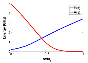
Plot of Single-Qubit Kinetic (Tunnelling) Energy (A) and Potential Energy Scale (B) over a Computation

Last, and definitely not least, 5,000 years of CPU time doesn’t just fall out of the sky.  We had to build up a community of volunteers interested in helping us on BOINC and make sure our app plays nicely with their computers.  They’re doing us a huge service, so the last thing we want is to be a burden.  To put things in perspective, I checked how much it’d cost to have done the same using rented server time on Amazon EC2, and it worked out to be around $4M to $5M, money we simply don’t have.

1. Pre-processing

One thing that we struggled with for ages was making sure that if we tell it to simulate something, it’s actually simulating that instead of it being in the process of heading toward simulating that so slowly that it never actually starts simulating the right thing.  That’s a very cryptic was of saying “it’s even hard to figure out where it should start”.

One part of the solution to this is to simply let it simulate for a while without looking at it, hoping that it’s heading toward a good starting location.  If you wait infinitely long, it will end up at a good location on average, but we don’t have that kind of time.  We used the fact that near the end of the computation, a successful computation will have the system near the correct solution to the problem, and farther from the end of the computation, the simulation can get into a rough approximation of the right distribution in a reasonable amount of time (a few minutes).

However, accurately sampling near a point in the computation where the simulation should be representing a superposition of two sets of states that are far apart from each other, e.g. when the gap in energy between the lowest two energy states is small, exactly the points we want to examine, isn’t easy.  If your simulation happens to fall into one of the two sets of states, (and usually one of the two is much easier to fall into than the other), it could take a very long time to randomly walk over to the other set, meaning that the simulation might only sample from one of the two, giving completely bogus results.

In order to get completely reliable results, we need to let the simulation make larger leaps… in a very controlled manner.  This is accomplished by having many copies of the system, each at a different point in the computation, able to swap with each other.  Carefully placing many more copies around these critical points where long distances need to be traversed is what Firas’ “Robust Parameter Selection” algorithm is all about.  It’s an improvement on an algorithm by a collaborator, Helmut Katzgraber, modified to handle even these very bad cases.  It’s still not perfect, since there are countless diabolical cases that can crop up, but with about a week of pre-processing on a half-dozen machines, it set up the bulk of the simulations in a round just fine.

2. Processing

A bunch of issues cropped up in the simulation’s main crunching, and a few of them require an intimate understanding of the theory behind it just to realize what to check.  One of them was a “free” parameter we hadn’t realized actually significantly impacted the accuracy of the simulation.  As it turns out, at one end of its possible range, almost any problem you give it to simulate will appear to be a trivial problem, whereas at the other end, it gives a very accurate simulation… but takes forever to simulate.  We had originally had it set to some value about halfway in between, where it was still quite inaccurate, but enough problems still appeared non-trivial that we didn’t clue in that something was wrong.  We happened to re-run a round of the simulations with a different value, and got drastically different results… curses!

So, in the end, we had to more than quadruple the size of our simulations to get accurate data, and to verify that the accuracy had roughly converged, we also ran a bunch of very slow simulations (about 4x as long again) of the smaller problems with 4x less error.

With all of this expansion in the simulation size, it’s a good thing we’d improved the performance of the app so much, or we’d simply have been sunk.  The following plot sums up some performance improvements, on top of improvements in the thread balancing, for the main crunching part of the app (which is now down to only about 34% of the time, so it’s no longer the bottleneck).

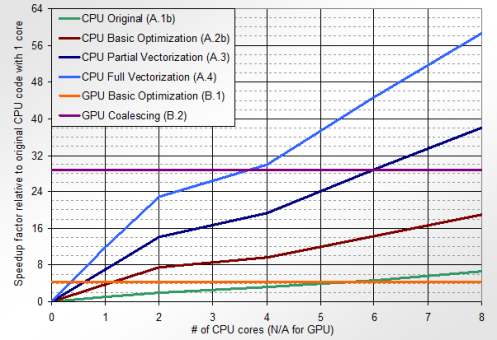
Main performance results from Importance of Explicit Vectorization for CPU and GPU Software Performance

3. Post-processing

I can’t fully express the pain of trying to sift through hundreds of thousands of huge output files trying to find ways of automatically identifying which ones represent bogus data (e.g. transmitted to/from a volunteers’ computer incorrectly, memory/disk corruption, spurious emergent behaviour in the random number generators, etc.)  Every output value has to be suspect.  There are a whole bunch of output values that are known to be exactly 1.0, and in the application, it’s numerically impossible for them to become any other value than 1.0.  Quite possibly the only reason these values are output at all is that in something like 1 in 500 output files (or more), one or more of these values is not 1.0.  Even if they’re 0.9999999 or 1.0000001, either some sort of memory or disk access was corrupted, or the CPU was computing simple operations incorrectly, or a user fiddled with the output data, etc.

Note that I have strong evidence that user tampering does not account for a majority of those errors, and not just because it would take a lot of effort and would get caught by my overly-suspicious post-processing checks.

Some other issues in post-processing included the combination and interpretation of extremely rough data.  It wasn’t just sufficient to handle noisy data, but even mediocre post-processing required estimation of the expected amount of noise on the data returned from the simulations.  That only took a few pages of scratch, but handling the dozens of special ways in which the noise can manifest itself took a few months off my lifespan.  Looking at the data as a human being with a brain, it’s usually so blatantly obvious where the noise kicks in, but trying to describe it for a computer to identify takes a lot of “patience”… actually, I don’t even need the air quotes, ’cause it takes a few hours to run the post-processing code and see if it worked or not.

A word of warning on the emergent behaviour in random number generators comment above, a negligibly small but non-zero probability can very easily accidentally become a 1 in 4,294,967,296 probability, which normally wouldn’t be an issue, but in huge simulations like these can cause maybe 1 in 200 output files to have a clearly unreasonable event occur that will throw off all results they’re used in.  That and random number generators may randomly happen to have the same seeds if you’re not careful.

Having a good way of visualizing the results was also critical in finding and understanding these issues.

Conclusion

This has been a heck of a challenge over the past year, and I’m glad the paper on it is finally out there, showing that the median adiabatic time is really negligible for many small problem instances.  There are much longer times that are more worthwhile worrying about in the mean time, e.g. milliseconds spent waiting for a chip to cool down after sending it a problem.

There are more exciting challenges going on with the Iterative QUANtum Algorithms (IQUANA) app, which uses results from one round of simulations to determine what happens on the next round… people don’t usually measure the time for one iteration of an algorithm in weeks, but this is an exception. 🙂

I can’t wait until the other big paper to be out soon is finally out.  That one took a solid 6 months mixed in there.

Multi-threading is Simple

A friend asked me to do a post on distributed/parallel computing.  Covering everything would be a bit much for one post, so I’d first like to address one of my biggest beefs related to multi-threading.

Specifically, many people have this bizarre assumption that multi-threading is difficult, perpetuated for no apparent reason by a few people who are evidently either too stubborn or too stupid to think and program at the same time (e.g. Joel Spolsky, the makers of SQLite).  I hope to show in this post that there’s very little excuse for not multi-threading, since you can do a half-decent job of it with one remarkably simple, general structure and almost no effort.

“Threads are evil. Avoid them.” –The SQLite FAQ

Multi-threading at its core is simple in concept and practice; people just never get a good explanation of how simple it can be, so understandably, they’ll tend to be mystified by it.  Perhaps the simplest way to view parallelism is on a dependency graph.  The following is an example of a dependency graph for a set of tasks to be done when planning a wedding:

Dependencies between some tasks for planning a wedding

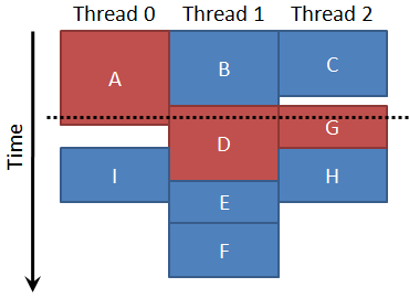
You can’t print invitations (task E) before you know the date (task C), otherwise the invitations might have the wrong date on them.  In other words, E depends on C.  Tasks that depend on each other can’t be run at the same time, because one must be done before the other.  However, tasks A, D, and G (in red) do not depend on each other, they are independent, so those 3 tasks could be done by different people at the same time, possibly saving time overall.  The following is one way that these tasks could be parallelized with 3 people/threads:

One possible parallelization of the above tasks with 3 people/threads

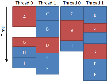
At all points in time, all tasks running at the same time must be independent.  Notice that when task C finishes, there is nothing ready to be run yet, so that thread can’t do anything until B finishes, when both G and D can be started.  This happens to be an optimal parallelization of these tasks, but supposing we only had 2 threads, here are 2 different parallelizations, one of which is not optimal:

Two different parallelizations of the above tasks with 2 people/threads

An interesting feature of these two parallelizations is that both of them are locally optimal, in that no single task can be moved to improve the total time in either case.

All this is well and good, but how exactly would we implement something like this?

This is also simple using a workpool.  A workpool is effectively any producer-consumer-like structure that represents tasks to be run.  One thread is created for each CPU core, and they each look for work in the pool.  This can sometimes be as simple as a single integer that is the index of the next task to be done in an array of completely independent tasks.  A workpool can even be completely implicit, such as when the entire being of what each thread is to do can be determined from their thread number (e.g. random sampling with each thread having a different seed, or each traversing a separate length of array).  However, any thread-level parallelism can be expressed in terms of just a workpool, though it is often much more efficient to use other control structures as well or alternatively.

The example above is actually one of the more complicated cases, where each task could have a list of tasks that depend on it (e.g. task G would have a list pointing to E, H, and I), and when the task finishes, it could decrement a counter on each of those tasks, indicating how many dependencies it’s waiting for.  If the number of dependencies some task is waiting for reaches zero, it can be added to the workpool.  Then, if there are any, some task from the workpool would be chosen to run in the current thread.

All of the above parallelizations can be obtained by that general workpool algorithm.

There are even some impressive properties that have been proven about workpools.  For example, if all of the tasks take the same time (in practice, if variation in task length is very small compared to the total time), any way of selecting tasks from the workpool will be at most 2x slower than the best, no matter what the dependencies, and on average, should be much better than that.  If there are few dependencies and a very large number of tasks, it becomes easy to obtain near-perfect speedup on many CPU cores.

There is a small caveat, for those paying close attention, and it’s from unintended dependencies.  For example, something as simple as decrementing the counter of how many tasks to wait for causes dependencies.  What if two threads try to decrement the counter at the same time?  Both read the value 5, subtract 1, and store the value 4, but if they’d been just a few clock cycles apart in timing, the value of the counter would be 3, since whichever one occurred second effectively depended on whichever one occurred first.  Worse yet is the multi-instruction operation of “adding a task to the workpool”.

This requires a mechanism for performing atomic operations, ones that cannot be divided into separate operations or overlapped by dependent operations.  Luckily, Intel and AMD provide an instruction prefix (the “lock” prefix) to make certain processor instructions atomic.  With these, we can construct multi-instruction atomic operations, a workpool, any other thread control mechanism, or even a thread scheduler, which doesn’t have the luxury of having its own thread.

Nonetheless, with just a functioning workpool implementation, it’s possible to do amazing stuff in parallel.  It very simply (i.e. 1 line of code and a bit of forethought) cuts down the post-processing time of AQUA@Home from over a day to a few hours on a Core i7 (8 logical CPU cores).  Workpools of some sort are also used in some form for all parallelism in the AQUA@Home applications.  With a careful way of selecting the next thing to run from a workpool, I can guarantee that one of the applications now spends at most ~10 seconds at the end not using all CPU cores 100%.  I also parallelized assembling down to the function level just by putting all the functions into a type of workpool in Inventor IDE.

I haven’t shown detail on a specific example here, but next time, I’ll walk through the parallelism of the main AQUA@Home application, presented in this paper I co-authored.

Importance of Explicit Vectorization for CPU and GPU Software Performance

The preprint version of my first paper as a lead author is now out here.  It’s been submitted to Parallel Computing for peer review.  The paper walks through several optimizations I did on the AQUA@Home Quantum Monte Carlo simulation code, independent of multi-threading.   The journal encourages authors to include multimedia too, so I’m looking into making brief tutorial videos (<5 minutes each) describing the optimizations.

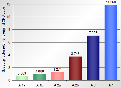
The upshot of the paper is mostly captured by Figure 13: 

Main performance results from Importance of Explicit Vectorization for CPU and GPU Software Performance

This compares an Intel Core i7-965 CPU and an NVIDIA GTX-285 GPU, both of which are currently close to the highest performance single processing units available from the respective companies.  For a more detailed look at the CPU versions, including two with compiler optimization off (A.1a and A.2a), Figure 15: 

Relative performance of CPU implementations at 6 different levels of optimization

The main conclusions are: 1) it is sometimes possible to achieve large speedups from explicitly optimizing code on both CPU and GPU, 2) it is sometimes possible for a CPU to outperform a GPU when both are running optimized code. 

CPU vs. GPU

I’ll start with the 2nd one, since it’s probably more controversial, and hence the most likely to result in angry emails or blog posts attacking my credibility.  How on earth can a high-end CPU with 8 logical cores outperform a high-end GPU with 240 cores by a factor of 2.04, when data transfer time is negligible?  This means that the performance of each CPU core would have to be comparable to the performance of 61.2 GPU cores in this application; a huge discrepancy to account for.  This  isn’t rigorous, but it goes through the primary factors involved.

Factor #1: Clock Speed.  The cores on the Intel Core i7 I used in the paper run at 3.2 GHz (I turned off overclocking, since it ironically made the graphics card flake out.)  The cores on the GTX-285 run at 648 MHz, faster than the GTX-295, in case you’re wondering.  That’s a factor of 4.94, still a discrepancy of 12.39x left.

Factor #2: Vector vs. Scalar.  Each core on the CPU spends the bulk of its time running instructions that do 4 operations at once on a vector.  Each GPU instruction only does 1 operation.  That factor of 4 leaves a discrepancy of 3.10x.

Factor #3: Branching.  In the scalar version of the code, there’s a key branch choosing whether or not to flip the sign of a variable and update data for related variables, which is taken 28.6% of the time on average.  However, if looking at 4 variables at once, if any one of them takes the branch, they must all wait, making the average probability 56.8% (computed from 115 separate probabilities, Figure 14, which is why it’s not ).  For the GPU, with groups of 32 threads (called warps) sharing an instruction pointer, they must wait 82.8% of the time.  This would be another factor of 1.46 (i.e. 82.8%/56.8%), but not all of the time is spent on that branch, so without knowing the breakdown of which parts took how long, one can’t be sure how much it contributes.

Factor #4: Clocks Per Instruction.  This is actually many factors, but difficult to separate.  The L3 cache on the Core i7 is 8MB, enough to hold some of the key data structures.  On the GTX-285, the similar “shared memory” on each multi-processor is only 16KB (and manually-controlled, unlike cache), meaning that the key data structures must reside in the “device memory”, which is considerably slower, analogous to main memory from the CPU’s perspective.  Also, each core of the Core i7 has multiple execution units, so it can be running multiple operations simultaneously, resulting in max throughput of 3 vector bit manipulation instructions in a single CPU clock cycle.  I couldn’t find reliable clock cycle numbers for the GTX-285, but each core has only one execution unit.

Although  factors #3 and #4 are not rigorous, they could reasonably account for the remaining 3.10x discrepancy.  Note that factors #3 and #4 are highly application-dependent, so it would be unwise to claim that this 61.2x core-per-core performance difference applies to more than this application, but one can at least account for a 19.75x difference, from factors #1 and #2, assuming the CPU code is vectorized.

To make sure it’s absolutely clear, I’m not stating that a CPU is generally faster than a GPU,  I’m stating that a GPU is not always faster than a CPU, and that comparing numbers of cores isn’t a good metric.

Explicit Performance Optimization

Many people I’ve talked to seem to think of performance optimization done explicity, i.e. in addition to implicit compiler optimization, as “beating the compiler”, or “performance tuning”, which I find quite frustrating.  You don’t get a 10x speedup by doing the same thing as the compiler only better; I’d go so far as to conjecture that compilers are good enough that you can’t get such a speedup that way.  The important thing to realize is that you have key knowledge that the compiler doesn’t have, such as “This code is just generating random numbers and can be replaced with faster code that would generate different random numbers.” or “It’s okay (and possible) to rearrange the order of these nodes so that groups of 4 adjacent nodes can be updated independently.”

As shown by the difference between A.1a and A.1b in the bar graph above, compiler optimizations gave a 1.51x speedup for the original code.  It’s certainly nothing to sneeze at when the simulations take months to run on over 2,000 computers, but by using knowledge about the problem and algorithm at hand, as well as about the CPU’s available computing resources, it was possible to get the final 11.86x speedup on top of that.  In implementation A.2a and A.2b, I wrote the random number generation code in a way that it would be easier for the compiler to vectorize, and it gave a 2.94x speedup from compiler optimizations instead of 1.51x, so it can vectorize when it’s given a chance.  I’m not “beating the compiler [at a fair fight]”, since the compiler doesn’t have a hope of guessing what I know about the problem, let alone using that knowledge.

This is one of the reasons why I find the term “optimizing compiler” rather outrageous.  It suggests to developers that there’s no point in optimizing, since the compiler’s already done it for them.  The claims made about compilers that automagically parallelize code are even more outrageous.

Conclusion

If you need your code to run much faster and can’t count on that many times more cores or computers, you may not be out of luck.

The Power of Optimization

People are pretty skeptical when I talk about getting big speedups from simple changes, so when optimizing/debugging the program I made recently to generate tough problem instances of Maximum Independent Set (MIS), I timed how long the generator took on one CPU core of my 1.66GHz Core 2 Duo laptop.

The program starts with a random graph that very likely has an independent set of size m, keeps the first independent set of size m that it finds, and adds edges as it searches so that the first one is the only independent set of size m.  There are many papers out there on hiding independent sets (or cliques) that are much larger than most in graphs, but this is the first I’ve heard of hiding an independent set that’s only one node larger than most of the maximal independent sets. I set out with the objective of getting 128-node graphs with a single maximum independent set of size 24.

The first version that worked correctly printed out every independent set it found, since I’d had some issues with correctly traversing the sets, so printing took a vast majority of the time.  Specifically:

nodes	initial edges	MIS size	build	printed	parameters passed	time (s)
32	64	12	32-bit debug	state, graph, and added edges	separately	~1200
32	64	12	32-bit debug	graph and added edges	separately	2.63
32	64	12	32-bit debug	added edges	separately	0.119
32	64	12	32-bit debug	none	separately	0.084
32	64	12	32-bit release	none	separately	0.037

This isn’t even doing any “real” optimizations; it was spending 99.997% of the time just printing out data. Speedup from not printing out anything and using release build: 32345x. In fact, the final result is so much shorter, that much of its time could be overhead, so the speedup on a larger instance would be higher.  I consider this like a design optimization, whereas the optimizations below are algorithmic optimizations.  I find that design optimizations usually have the largest impact and result in simpler code, though in this case the code wasn’t really much simpler since it wasn’t really a full-out design change.  Design changes are almost always of the type “I don’t need to do all this stuff… why am I doing it anyway?”  Moral of the story: printing text is ridiculously slow; avoid unnecessary logging.

Now that it was so much faster, I needed a larger test case, so I started ramping up the graph size:

nodes	initial edges	MIS size	build	printed	parameters	time (s)
64	400	16	32-bit release	none	separately	4.33
96	640	20	32-bit release	none	separately	~2316
96	640	20	32-bit release	none	together	~2598

This was the first “real” optimization I tried, and it didn’t work. The search is highly recursive and has 10 parameters, most of which don’t change, so I was thinking that passing them together in a structure would be better, but it wasn’t. The overhead of accessing them indirectly outweighted the savings from only passing 4 parameters. Moral of the story: even for functions with a ton of parameters, function calling is fast; it’s the content of the function that matters… as long as it isn’t a tiny function.

At this point, I went for a trick I’d done before for traversing independent sets, but I wasn’t sure how it’d work in this case, since it has to add edges too. The trick is whenever the number of nodes left that could be added to the current set is 64 or less, I bit-pack the adjacency matrix for the subgraph induced by these nodes and operate on entire rows of the matrix at once, since each row fits into a qword (unsigned long long). With a 64-bit build, this can be done quite efficiently. It took a lot of debugging to get this to work properly, but it was worth it:

nodes	initial edges	MIS size	build	printed	parameters	other	time (s)
96	640	20	64-bit debug	added edges	separately	64-node trick, error-checking	54.6
96	640	20	64-bit release	none	separately	64-node trick	18.4
128	1200	24	64-bit release	none	separately	64-node trick	~666

That did the trick. It was now possible to accomplish the objective of getting a 128-node graph with a unique MIS of size 24 in just over 11 minutes. Speedup from bit-packing, to do many operations in parallel and reduce overhead: 126x. Moral of the story: simple bit operations take a clock cycle or two; fiddling around with data structures usually takes much longer. This still wasn’t quite where I wanted it, since now that it seems feasible, I would like to ramp it up a bit more. Luckily, I could easily improve the early cut-off check I had (i.e. when there aren’t enough nodes left to create an independent set of size m, you can avoid looking there.)

nodes	initial edges	MIS size	build	printed	parameters	other	time (s)
128	1200	24	64-bit release	none	separately	64-node trick & early cut-off	134
128	900	32	64-bit release	none	separately	64-node trick & early cut-off	811

That helped too. Speedup from early cut-off: 5x. Moral of the story: don’t compute things that you don’t need to, as long as it’s easy to check whether you need to compute them or not.

Final speedup: 625x from just algorithmic optimizations. 20 million x total. To generate 50 graphs of the last type, it’ll only take 11.3 CPU-hours now, but it’d have taken 293 CPU-days without any optimization other than removing printing and using a release build.  I haven’t done any detail-level optimization, what most people call “inner-loop optimization”.  I could do a bunch more, i.e. this is still single-threaded and in C; I could do much better in assembly language and with 8 threads on the Intel Core i7 CPU at work. I’ll probably generate 8 graphs at once by adding a simple OpenMP parallel for loop. However, there’s not much use in generating such graphs with more than 128 nodes at the moment, so I’m back to working on a secret side project I hope you’ll like. 🙂

Proof for a Post a While Back

In a post a while back, I mentioned that I’d found that:

for sufficiently large k, which relates to finding the median of the minimum of a set of k independent, identically-distributed random variables.  I didn’t have a proof at the time, but I’ve thought of a very simple “proof”:

for large x.

It’s by no means rigorous, as things that are “approximately equal” put through certain transformations can result in values that  are not even close, but it seems to check out in this case.

Roots of Two and the Median of the Minimum

Yet another weird math observation.  As k becomes large (like k=1000 has less than 0.034% relative error):

I haven’t actually looked into why this is, but it means that:

So why am I looking at this?  Well, I’m really looking at the finding the median of the minimum of k independent, identically-distributed random varaibles.  With k such variables:

The question is, what value a is the median of the minimum?  Let’s define and solve for it:

If it’s the minimum of many independent variables, it’s then .  So, as long as we can find the value a at percentile p of the original distribution, we’ve found the median of this distribution of the minimum.  Weird stuff.

Inventor IDE Alpha 5b Released, but…

So technically Inventor IDE Alpha 5b is now released on codecortex.com; the problem is that nobody can access codecortex.com right now, even though the bill got paid in time thanks to my father.  Well, I’ll just hope that it gets resolved soon and say a bit about this release.

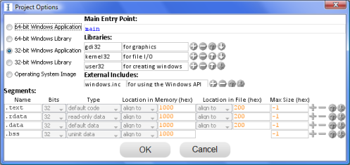
This release finally lets users create 64-bit applications and operating system images by selecting them in the new project options dialog:

Project Options Dialog Box

There are also many user interface improvements that probably nobody else will notice, but that will come in handy in the next videos of the tutorial I’ll be continuing again soon.  One that people may notice is one that I’d wanted to avoid, but there is now a progress bar for loading.  Personally, I wanted the loading performance to be improved to the point there that wasn’t needed, but that’ll have to wait for the Beta version.

There are some encoding bugs fixed, mostly for the support for 64-bit code, inline functions, and not-yet-released performance test functions.  As an example it turns out that general registers r12 and r13 need some undocumented encodings that I hadn’t supported until today.

The next things potentially on the agenda for Alpha 6 releases are:

• Find/replace bar, a twist on the classic find bar
• Find all references
• Unit/performance testing system
• Exports & relocations, to really support making libraries
• Listing files (a request from Prof. Reichstein for COMP 2003, and something that’d help debugging operating system code)
• Navigation side strip, for quick navigation within a file, especially for errors
• Output formats: OBJ, LIB, ELF, and Mach-O, to support Windows, Linux, and Mac with the same source code
• Input OBJs or LIBs

Things higher up are currently more likely to come sooner, but if people have any requests, please let me know.  The most likely is that only a few will get implemented for Alpha 6, and the rest will be put off for when Inventor IDE has been ported to C/C++.